
Presentation of the game
The power game 4 comes in the form of a game board, with 7 (horizontal) x 6 (vertical) circular openings, where different colored tokens are stacked.
Two players compete against each other with the objective of being able to line up, the first, 4 tokens of the same color, horizontally, vertically or diagonally. Each player successively slides his token.
Although the number of combinations is much smaller than the game of go (1,5.1013 possible combinations), and it was solved exactly in 1988, by James D. Allen, and independently by Victor Allis, this last algorithm nevertheless makes it possible, with a reasonable computing power, to give a concrete application.
In order to model the game in Python and to implement the MCTS algorithm we will mainly use two packages, Numpy to simulate the game board, and Anytree to build the tree needed for the MCTS.
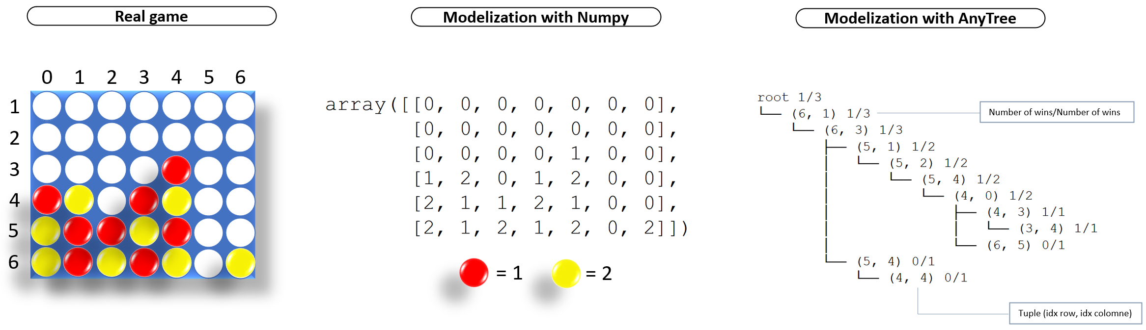
To simplify the modeling of the game, we will use a null matrix 06, 7 with Numpy, the red and yellow pawns will correspond respectively to “1” and “2” in the Numpy matrix and the “0” to empty places. On AnyTree each node of the tree will be identified by its index.
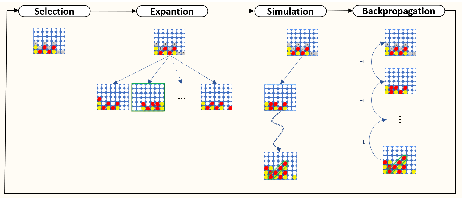
- Selection :
The MCTS has a major advantage, it selects beforehand in a clever way each action according to the state and knowledge of the game that it acquires as it goes along.
This first step, on the one hand, tries to identify the available actions, in our case it is a question here of identifying all the spaces available to play a token, and on the other hand, to identify the most suitable location. more interesting to explore. A compromise is then defined between the benefit of exploration and optimal game so far known.
This compromise is fixed by the following formula UCB 1
\(\fbox{$X_j+c\sqrt{\frac{ln\,n }{n_j}}$}\)
- Xj is the average reward for j
- nj is number of times j has been played
- n is the total number of games played
- c is the exploration parameter – usually equal to √2
def UCB1(val):
   ucb1={}
    for i in val.keys():
       if val[i]["children"]["nb_visit"]==0:
          ucb1[i]=np.inf
       else :
          val_ucb1=val[i]["children"]["nb_win"]/val[i]["children"]["nb_visit"]+np.sqrt(2)*np.sqrt(np.log(val[i]["parent"]["nb_visit"])/val[i]["children"]["nb_visit"]) ucb1[i]=val_ucb1
 return ucb1
An analysis of this formula, shows us that if a child node has a much higher value than the others, this child node will be explored much more often than the others, UCB1 most of the time selects the “max” child node. However, if two child nodes have a similar value, the results of the function will be close. Finally, a node not at all explored will have priority with a default value of + ∞. This game strategy ultimately leads to the tree growing asymmetrically and exploring good moves more deeply.
- Expantion :
Once the place to explore is identified, we simulate a game, randomly from that target node. Note that nodes visited during this random simulation are not saved.
To boost the performance of the tree search, we can create an intelligent agent, with which we will compare it. Like a Monte Carlos Simple, which would simulate a large number of games, and which after simulation would tell the agent where to play. Or something simpler like a trivial agent that would play randomly most of the time. But could identify the states of the game where he would have or the opponent would have three tokens lined up in order to block or play the winning move. (Available in code)
def expantion(game_tree,state,available_play):
    node_val={}
    for i in available_play:
        state_tmp=state.copy()
        path=search.findall_by_attr(game_tree ,i)
        state_tmp.append(i)

        if path==():
            node_val[i]={"parent":{"nb_win":0,"nb_visit":0},"children":{"nb_win":0,"nb_visit":0}}


        else:
            for z in range(len(path)):

                if [node.name for node in path[z].path]==state_tmp:

                    node_val[i]={"parent":{"nb_win":0,"nb_visit":0},"children":{"nb_win":0,"nb_visit":0}}
                    node_val[i]["parent"]={"nb_win":path[z].parent.nb_win,"nb_visit":path[z].parent.nb_visit}
                    node_val[i]["children"]={"nb_win":path[z].nb_win,"nb_visit":path[z].nb_visit}


                elif i not in node_val:

                    node_val[i]={"parent":{"nb_win":0,"nb_visit":0},"children":{"nb_win":0,"nb_visit":0}}

    return  node_val
- Backpropagation :
The operation of Backpropagation consists in updating the tree which contains all the games played. At the end of each game, each node through which a token has been played is updated: the nb_visit field is incremented by one, as well as the nb_win field if the game results in a victory.
def update_tree(game_tree,game_lst):

    root_name = game_lst[0][0][0]
    for branch, result  in zip([x for x,_ in game_lst],[x[1] for x in game_lst]):
        parent_node = game_tree
        assert branch[0] == parent_node.name
        for cur_node_name in branch[1:]:
            cur_node = next(
                (node for node in parent_node.children if node.name == cur_node_name),
                None,
            )


            if cur_node is None:
                cur_node = Node(cur_node_name, parent=parent_node,nb_visit=0,nb_win=0)

            parent_node = cur_node

        #backpropagation
        for i in list(cur_node.iter_path_reverse()):
            i.nb_win=i.nb_win+result
            i.nb_visit=i.nb_visit+1

    return game_tree
The above function, takes two parameters as input: “game_lst” which contains a list of tuple which corresponds to a game, the tuples correspond to the index of tokens to play. This function also takes the tree of the different games already simulated “game_tree”. As a response, this function will return this updated tree.
You will find all the code on github here
Références
[1] SILVER, David, HUANG, Aja, MADDISON, Chris J., et al. Mastering the game of Go with deep neural networks and tree search. nature, 2016, vol. 529, no 7587, p. 484-489. [link]
[2] Victor Allis . A Knowledge-Based Approach of Connect Four: The Game is Over, White to Move Wins,1988, M.Sc. Thesis, Report No. IR-163, Faculty of Mathematics and Computer Science, [link]